

Fashion MNIST classification using custom PyTorch Convolution Neural Network (CNN)
Hi, in today’s post we are going to look at image classification using a simple PyTorch architecture. We’re going to use the Fashion-MNIST data, which is a famous benchmarking dataset. Below is a brief summary of the Fashion-MNIST.
Fashion-MNIST is a dataset of Zalando’s article images—consisting of a training set of 60,000 examples and a test set of 10,000 examples. Each example is a 28x28 grayscale image, associated with a label from 10 classes. Zalando intends Fashion-MNIST to serve as a direct drop-in replacement for the original MNIST dataset for benchmarking machine learning algorithms. It shares the same image size and structure of training and testing splits.
The original MNIST dataset contains a lot of handwritten digits. Members of the AI/ML/Data Science community love this dataset and use it as a benchmark to validate their algorithms. In fact, MNIST is often the first dataset researchers try. “If it doesn’t work on MNIST, it won’t work at all”, they said. “Well, if it does work on MNIST, it may still fail on others.”
The Fashion-MNIST can be cloned from the following GitHub repo and please don’t forget to check out the Fashion-MNIST paper for more detials.
Each of the labels in the data will correspond to either one of the following classes;
<!DOCTYPE html>
Fashion-MNIST labels
| class | label |
|---|---|
| T-shirt/top | 0 |
| Trouser | 1 |
| Pullover | 2 |
| Dress | 3 |
| Coat | 4 |
| Sandal | 5 |
| Shirt | 6 |
| Sneaker | 7 |
| Bag | 8 |
| Ankle boot | 9 |
# import some dependencies
import torchvision
import torch
import torchvision.transforms as transforms
import numpy as np
import matplotlib.pyplot as plt

import torch.optim as optim
import time
import torch.nn as nn
import torch.nn.functional as F
torch.set_printoptions(linewidth=120)
# import data
train_set = torchvision.datasets.FashionMNIST(root="./", download=True,
                                              train=True,
                                              transform=transforms.Compose([transforms.ToTensor()]))

test_set = torchvision.datasets.FashionMNIST(root="./", download=True,
                                              train=False,
                                              transform=transforms.Compose([transforms.ToTensor()]))
data_loader = torch.utils.data.DataLoader(train_set, batch_size=10, shuffle=True)
sample = next(iter(data_loader))

imgs, lbls = sample
visualize some samples
# create a grid
plt.figure(figsize=(15,10))
grid = torchvision.utils.make_grid(nrow=20, tensor=imgs)
print(f"image tensor: {imgs.shape}")
print(f"class labels: {lbls}")
plt.imshow(np.transpose(grid, axes=(1,2,0)), cmap='gray');
image tensor: torch.Size([10, 1, 28, 28])
class labels: tensor([8, 0, 9, 9, 7, 5, 9, 5, 2, 6])
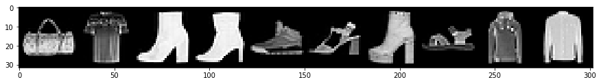
As we can see from the above, the images are grayscale 28 by 28 images. Without further ado, lets define a simple network that will learn to map the inputs (images) to the correct class (label/target). To do this we will be using a classic way to program a neural network (i.e, using object oriented programming or OOP), train it over a few epochs (iterations) and inspect the results using a confusion matrix. Before we do this, lets define some functions we will be using..
# define some helper functions
def get_item(preds, labels):
    """function that returns the accuracy of our architecture"""
    return preds.argmax(dim=1).eq(labels).sum().item()

@torch.no_grad() # turn off gradients during inference for memory effieciency
def get_all_preds(network, dataloader):
    """function to return the number of correct predictions across data set"""
    all_preds = torch.tensor([])
    model = network
    for batch in dataloader:
        images, labels = batch
        preds = model(images) # get preds
        all_preds = torch.cat((all_preds, preds), dim=0) # join along existing axis

    return all_preds


def plot_confusion_matrix(cm,
                          target_names,
                          title='Confusion matrix',
                          cmap=None,
                          normalize=True):
    """
    given a sklearn confusion matrix (cm), make a nice plot

    Arguments
    ---------
    cm:           confusion matrix from sklearn.metrics.confusion_matrix

    target_names: given classification classes such as [0, 1, 2]
                  the class names, for example: ['high', 'medium', 'low']

    title:        the text to display at the top of the matrix

    cmap:         the gradient of the values displayed from matplotlib.pyplot.cm
                  see http://matplotlib.org/examples/color/colormaps_reference.html
                  plt.get_cmap('jet') or plt.cm.Blues

    normalize:    If False, plot the raw numbers
                  If True, plot the proportions

    Usage
    -----
    plot_confusion_matrix(cm           = cm,                  # confusion matrix created by
                                                              # sklearn.metrics.confusion_matrix
                          normalize    = True,                # show proportions
                          target_names = y_labels_vals,       # list of names of the classes
                          title        = best_estimator_name) # title of graph

    Citiation
    ---------
    http://scikit-learn.org/stable/auto_examples/model_selection/plot_confusion_matrix.html

    """
    import matplotlib.pyplot as plt
    import numpy as np
    import itertools

    accuracy = np.trace(cm) / np.sum(cm).astype('float')
    misclass = 1 - accuracy

    if cmap is None:
        cmap = plt.get_cmap('Blues')

    plt.figure(figsize=(15, 10))
    plt.imshow(cm, interpolation='nearest', cmap=cmap)
    plt.title(title)
    plt.colorbar()

    if target_names is not None:
        tick_marks = np.arange(len(target_names))
        plt.xticks(tick_marks, target_names, rotation=45)
        plt.yticks(tick_marks, target_names)

    if normalize:
        cm = cm.astype('float') / cm.sum(axis=1)[:, np.newaxis]


    thresh = cm.max() / 1.5 if normalize else cm.max() / 2
    for i, j in itertools.product(range(cm.shape[0]), range(cm.shape[1])):
        if normalize:
            plt.text(j, i, "{:0.4f}".format(cm[i, j]),
                     horizontalalignment="center",
                     color="white" if cm[i, j] > thresh else "black")
        else:
            plt.text(j, i, "{:,}".format(cm[i, j]),
                     horizontalalignment="center",
                     color="white" if cm[i, j] > thresh else "black")


    plt.tight_layout()
    plt.ylabel('True label')
    plt.xlabel('Predicted label\naccuracy={:0.4f}; misclass={:0.4f}'.format(accuracy, misclass))
    plt.show()
# define network

class Network(nn.Module): # extend nn.Module class of nn
    def __init__(self):
        super().__init__() # super class constructor
        self.conv1 = nn.Conv2d(in_channels=1, out_channels=6, kernel_size=(5,5))
        self.batchN1 = nn.BatchNorm2d(num_features=6)
        self.conv2 = nn.Conv2d(in_channels=6, out_channels=12, kernel_size=(5,5))
        self.fc1 = nn.Linear(in_features=12*4*4, out_features=120)
        self.batchN2 = nn.BatchNorm1d(num_features=120)
        self.fc2 = nn.Linear(in_features=120, out_features=60)
        self.out = nn.Linear(in_features=60, out_features=10)


    def forward(self, t): # implements the forward method (flow of tensors)

        # hidden conv layer
        t = self.conv1(t)
        t = F.max_pool2d(input=t, kernel_size=2, stride=2)
        t = F.relu(t)
        t = self.batchN1(t)

        # hidden conv layer
        t = self.conv2(t)
        t = F.max_pool2d(input=t, kernel_size=2, stride=2)
        t = F.relu(t)

        # flatten
        t = t.reshape(-1, 12*4*4)
        t = self.fc1(t)
        t = F.relu(t)
        t = self.batchN2(t)
        t = self.fc2(t)
        t = F.relu(t)

        # output
        t = self.out(t)

        return t
cnn_model = Network() # init model
print(cnn_model) # print model structure
Network(
  (conv1): Conv2d(1, 6, kernel_size=(5, 5), stride=(1, 1))
  (batchN1): BatchNorm2d(6, eps=1e-05, momentum=0.1, affine=True, track_running_stats=True)
  (conv2): Conv2d(6, 12, kernel_size=(5, 5), stride=(1, 1))
  (fc1): Linear(in_features=192, out_features=120, bias=True)
  (batchN2): BatchNorm1d(120, eps=1e-05, momentum=0.1, affine=True, track_running_stats=True)
  (fc2): Linear(in_features=120, out_features=60, bias=True)
  (out): Linear(in_features=60, out_features=10, bias=True)
)
# let's also normalize the data for faster convergence

# import data
mean = 0.2859;  std = 0.3530 # calculated using standization from the MNIST itself which we skip in this blog
train_set = torchvision.datasets.FashionMNIST(root="./", download=True,
                                              transform=transforms.Compose([transforms.ToTensor(),
                                                                            transforms.Normalize(mean, std)
                                                                           ]))
data_loader = torch.utils.data.DataLoader(train_set, batch_size=100, shuffle=True, num_workers=1)
optimizer = optim.Adam(lr=0.01, params=cnn_model.parameters())
# def train loop

for epoch in range(5):
    start_time = time.time()
    total_correct = 0
    total_loss = 0
    for batch in data_loader:
        imgs, lbls = batch
        preds = cnn_model(imgs) # get preds
        loss = F.cross_entropy(preds, lbls) # compute loss
        optimizer.zero_grad() # zero grads
        loss.backward() # calculates gradients
        optimizer.step() # update the weights

        total_loss += loss.item()
        total_correct += get_item(preds, lbls)
        accuracy = total_correct/len(train_set)
    end_time = time.time() - start_time
    print("Epoch no.",epoch+1 ,"|accuracy: ", round(accuracy, 3),"%", "|total_loss: ", total_loss, "| epoch_duration: ", round(end_time,2),"sec")
Epoch no. 1 |accuracy:  0.829 % |total_loss:  276.2480258792639 | epoch_duration:  80.73 sec
Epoch no. 2 |accuracy:  0.871 % |total_loss:  206.40078330039978 | epoch_duration:  70.3 sec
Epoch no. 3 |accuracy:  0.883 % |total_loss:  190.10711652040482 | epoch_duration:  73.01 sec
Epoch no. 4 |accuracy:  0.891 % |total_loss:  175.60668615996838 | epoch_duration:  83.73 sec
Epoch no. 5 |accuracy:  0.899 % |total_loss:  165.3020654693246 | epoch_duration:  111.66 sec
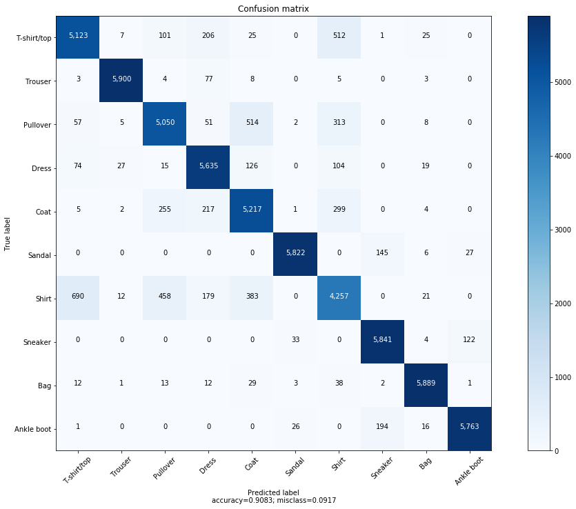
- training is complete, it’s time to inspect how well our algorithm performed using the confusion matrix!
train confusion matrix
# get all preds
pred_data_loader = torch.utils.data.DataLoader(batch_size=10000, dataset=train_set, num_workers=1)
all_preds= get_all_preds(network=cnn_model, dataloader=pred_data_loader)
plot_confusion_matrix(cm=confusion_matrix(y_true=train_set.targets, y_pred=all_preds.argmax(1)), target_names=train_set.classes, normalize=False)
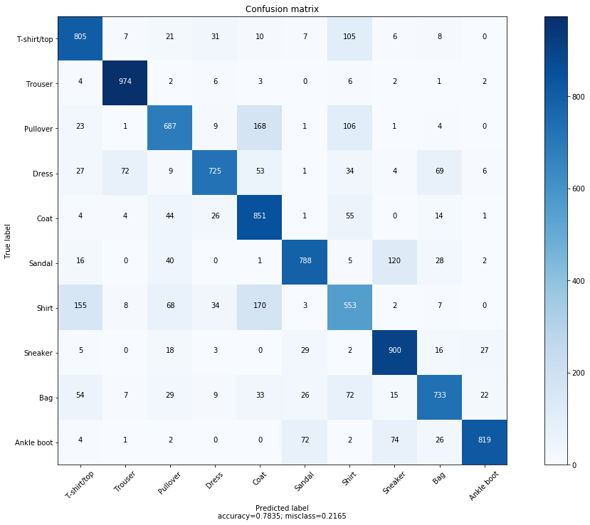
test confusion matrix (out of sample performance)
# get all preds
test_pred_data_loader = torch.utils.data.DataLoader(batch_size=10000, dataset=test_set, num_workers=1)
all_preds_test = get_all_preds(network=cnn_model, dataloader=test_pred_data_loader)
plot_confusion_matrix(cm=confusion_matrix(y_true=train_set.targets, y_pred=all_preds_test.argmax(1)), target_names=test_set.classes, normalize=False)
Conclusion
- model was slightly overfit
- train accuracy was about 90% while the test accuracy was 78%
- We could train for more epochs, however, the BN-CNN performed well but results could be improved with transfer learning, which will be the future of this work.
Thanks to the following for providing insights!
- support community at deeplizard
- Zilando for making Fashion-MNIST open access for testing code such as this!