
Bangalorehouseprediction

Housing situation in Bangalore, India.
Housing has increasingly become a basic need for every human being. This mini paper aims to provide insight into this essential requirement by exploring and analyzing the housing property market in Bangalore. Often referred to as the “Silicon Valley of India,” Bangalore is the state capital of Karnataka. Located in the southern part of the country, the city is home to over 10 million people, making it the third most populous city in India. As the nation’s chief technology hub and a major exporter, Bangalore offers a wealth of employment opportunities, which in turn places significant pressure on the housing market.
This situation is not surprising, as large cities tend to attract individuals seeking better jobs and higher incomes. According to Sheikh [1], the property market in India differs greatly from that of the rest of the world due to its rapid growth and other unique factors. However, determining property value can be complex, as it is not immediately clear what drives the cost of residential real estate in a large, developed city. While budget is an important consideration when purchasing property, it is equally important to understand the preferences and priorities that influence residential buyers.
This mini paper examines several variables—including area type, availability, location, size, society, total square footage, number of bathrooms, balcony availability, and price—to better understand the housing scenario in Bangalore.
Problem statement
Buying a home in Bangalore is especially a tricky choice. Buyer choice can be inspired by different aspects as such it’s difficult to ascertain property price. This leads to the question, what characteristics does a potential residence buyer consider before making purchase? The answer to this question will give us an understanding into the buyer dynamics in the metro of Bangalore.
Hypothesis
Since Bangalore is a silicon valley with a slew of opportunities for many Indians it’s more reasonable to think that people will find it pleasant to live just about anywhere. We hypothesize that the number of rooms has no effect on the sale price.
Data source
The data to be used were curated by a specialized team in India over months of primary and secondary research. The data are also publicly available online and distributed under the creative commons license on the Kaggle platform [3]. The variables under scrutiny are either categorical or continuous and cover details like; the area type which describes the type build in an area. Availability which indicates whether a house is available for possession or when it will be ready. Location which tells us where the residential property is situated in the metro. For example, along an airport highway. Price, which tells us the commercial value of the asset in lakhs or Indian rupee. Size, which refers to the number of bedrooms in a particular residential property. Bath tells us how many bath rooms a residence. Total square feet which gives a hint at the area the property occupies. The remaining variables like balcony and society detail how many balconies are on a property and which social group the property belongs.
Method
After acquiring the the data, the next steps will be to clean it (remove any outliers, convert any categorical variables one hot encoded vectors), understand the variables (their distributions) , perform some inferential statistics and lastly perform predictive modeling using linear regression. The software environment for this project will be python using an IDE or Integrated development environment (python interpreter).
Now let’s jump right into the code!
# import convinience functions

import pandas as pd
import matplotlib.pyplot as plt
import numpy as np
import seaborn as sns

# statistic package
import scipy.stats as stats
from statsmodels.stats.weightstats import ztest
import math

import warnings
warnings.filterwarnings(action="ignore") # turn off warnings

# import learners and other dependancies
from sklearn.model_selection import train_test_split
from sklearn.cross_validation import cross_val_score, ShuffleSplit
from sklearn.linear_model import LinearRegression, ridge_regression
from sklearn.tree import DecisionTreeRegressor
from sklearn.ensemble import RandomForestRegressor
np.random.seed(seed=123)


%matplotlib inline
# import data and read first 5 rows
df = pd.read_csv("Bengaluru_House_Data.csv")
df.head()
| area_type | availability | location | size | society | total_sqft | bath | balcony | price | |
|---|---|---|---|---|---|---|---|---|---|
| 0 | Super built-up Area | 19-Dec | Electronic City Phase II | 2 BHK | Coomee | 1056 | 2.0 | 1.0 | 39.07 |
| 1 | Plot Area | Ready To Move | Chikka Tirupathi | 4 Bedroom | Theanmp | 2600 | 5.0 | 3.0 | 120.00 |
| 2 | Built-up Area | Ready To Move | Uttarahalli | 3 BHK | NaN | 1440 | 2.0 | 3.0 | 62.00 |
| 3 | Super built-up Area | Ready To Move | Lingadheeranahalli | 3 BHK | Soiewre | 1521 | 3.0 | 1.0 | 95.00 |
| 4 | Super built-up Area | Ready To Move | Kothanur | 2 BHK | NaN | 1200 | 2.0 | 1.0 | 51.00 |
print(f"The dataset has {df.shape[0]} observations")
The dataset has 13320 observations
- There are some ethical issues to consider so we make a simple assumption that when a house will be available, the society it belongs to, the number of balconies and it’s area type will not be used to determine the final price.
cols_to_drop = [
    "area_type",
    "availability",
    "society",
    "balcony"
]
df_final = df.drop(columns=cols_to_drop)
df_final.head()
| location | size | total_sqft | bath | price | |
|---|---|---|---|---|---|
| 0 | Electronic City Phase II | 2 BHK | 1056 | 2.0 | 39.07 |
| 1 | Chikka Tirupathi | 4 Bedroom | 2600 | 5.0 | 120.00 |
| 2 | Uttarahalli | 3 BHK | 1440 | 2.0 | 62.00 |
| 3 | Lingadheeranahalli | 3 BHK | 1521 | 3.0 | 95.00 |
| 4 | Kothanur | 2 BHK | 1200 | 2.0 | 51.00 |
Data cleaning
df_final.isna().sum() # check the number of missing values
location       1
size          16
total_sqft     0
bath          73
price          0
dtype: int64
- the observation here is that we have very few missing values compare to 13000 observations so we can just drop them to make the analysis simpler
df_final.dropna(inplace=True) # drop missing values
df_final.head()
| location | size | total_sqft | bath | price | |
|---|---|---|---|---|---|
| 0 | Electronic City Phase II | 2 BHK | 1056 | 2.0 | 39.07 |
| 1 | Chikka Tirupathi | 4 Bedroom | 2600 | 5.0 | 120.00 |
| 2 | Uttarahalli | 3 BHK | 1440 | 2.0 | 62.00 |
| 3 | Lingadheeranahalli | 3 BHK | 1521 | 3.0 | 95.00 |
| 4 | Kothanur | 2 BHK | 1200 | 2.0 | 51.00 |
- upon droping missing values, we oberve that size has a wierd naming skim
- we can inspect this and find a way to correct it
df_final["size"].unique()
array(['2 BHK', '4 Bedroom', '3 BHK', '4 BHK', '6 Bedroom', '3 Bedroom',
       '1 BHK', '1 RK', '1 Bedroom', '8 Bedroom', '2 Bedroom',
       '7 Bedroom', '5 BHK', '7 BHK', '6 BHK', '5 Bedroom', '11 BHK',
       '9 BHK', '9 Bedroom', '27 BHK', '10 Bedroom', '11 Bedroom',
       '10 BHK', '19 BHK', '16 BHK', '43 Bedroom', '14 BHK', '8 BHK',
       '12 Bedroom', '13 BHK', '18 Bedroom'], dtype=object)
# we can use a simple function to remove the number of rooms from the column "size"
df_final["BHK"] = df_final["size"].apply(lambda x : int(x.split(" ")[0])) # convert no. of rooms to int
df_final = df_final[['location', 'size','BHK', 'total_sqft', 'bath',  'price']] # re-arrange cols
df_final.head()
| location | size | BHK | total_sqft | bath | price | |
|---|---|---|---|---|---|---|
| 0 | Electronic City Phase II | 2 BHK | 2 | 1056 | 2.0 | 39.07 |
| 1 | Chikka Tirupathi | 4 Bedroom | 4 | 2600 | 5.0 | 120.00 |
| 2 | Uttarahalli | 3 BHK | 3 | 1440 | 2.0 | 62.00 |
| 3 | Lingadheeranahalli | 3 BHK | 3 | 1521 | 3.0 | 95.00 |
| 4 | Kothanur | 2 BHK | 2 | 1200 | 2.0 | 51.00 |
# let's inspect the number of rooms
df_final["BHK"].unique()
array([ 2,  4,  3,  6,  1,  8,  7,  5, 11,  9, 27, 10, 19, 16, 43, 14, 12,
       13, 18])
- some houses have 43 bedrooms. It would also be interesting to look at the total sqft occupied by these kind of houses with more than 10 rooms and see if there is any relationship.
df_final[df_final["BHK"]>10]
| location | size | BHK | total_sqft | bath | price | |
|---|---|---|---|---|---|---|
| 459 | 1 Giri Nagar | 11 BHK | 11 | 5000 | 9.0 | 360.0 |
| 1718 | 2Electronic City Phase II | 27 BHK | 27 | 8000 | 27.0 | 230.0 |
| 1768 | 1 Ramamurthy Nagar | 11 Bedroom | 11 | 1200 | 11.0 | 170.0 |
| 3379 | 1Hanuman Nagar | 19 BHK | 19 | 2000 | 16.0 | 490.0 |
| 3609 | Koramangala Industrial Layout | 16 BHK | 16 | 10000 | 16.0 | 550.0 |
| 3853 | 1 Annasandrapalya | 11 Bedroom | 11 | 1200 | 6.0 | 150.0 |
| 4684 | Munnekollal | 43 Bedroom | 43 | 2400 | 40.0 | 660.0 |
| 4916 | 1Channasandra | 14 BHK | 14 | 1250 | 15.0 | 125.0 |
| 6533 | Mysore Road | 12 Bedroom | 12 | 2232 | 6.0 | 300.0 |
| 7979 | 1 Immadihalli | 11 BHK | 11 | 6000 | 12.0 | 150.0 |
| 9935 | 1Hoysalanagar | 13 BHK | 13 | 5425 | 13.0 | 275.0 |
| 11559 | 1Kasavanhalli | 18 Bedroom | 18 | 1200 | 18.0 | 200.0 |
- it is questionable if a house of 43 bedrooms will have 40 bathrooms and also if occupying a total area of 2400 makes much sense?
df_final["total_sqft"].unique()
array(['1056', '2600', '1440', ..., '1133 - 1384', '774', '4689'],
      dtype=object)
- some of the values in total_sqft are represented in a range, we might need a single value for this. Let’s take the avarage of such instances
df = df_final.copy()
def is_float(x):
    try:
        float(x)
    except:
        return False
    return True
df[~df["total_sqft"].apply(is_float)].head(10)
| location | size | BHK | total_sqft | bath | price | |
|---|---|---|---|---|---|---|
| 30 | Yelahanka | 4 BHK | 4 | 2100 - 2850 | 4.0 | 186.000 |
| 122 | Hebbal | 4 BHK | 4 | 3067 - 8156 | 4.0 | 477.000 |
| 137 | 8th Phase JP Nagar | 2 BHK | 2 | 1042 - 1105 | 2.0 | 54.005 |
| 165 | Sarjapur | 2 BHK | 2 | 1145 - 1340 | 2.0 | 43.490 |
| 188 | KR Puram | 2 BHK | 2 | 1015 - 1540 | 2.0 | 56.800 |
| 410 | Kengeri | 1 BHK | 1 | 34.46Sq. Meter | 1.0 | 18.500 |
| 549 | Hennur Road | 2 BHK | 2 | 1195 - 1440 | 2.0 | 63.770 |
| 648 | Arekere | 9 Bedroom | 9 | 4125Perch | 9.0 | 265.000 |
| 661 | Yelahanka | 2 BHK | 2 | 1120 - 1145 | 2.0 | 48.130 |
| 672 | Bettahalsoor | 4 Bedroom | 4 | 3090 - 5002 | 4.0 | 445.000 |
def convert_sqft_to_num(x):
    tokens = x.split("-")
    if len(tokens) == 2:
        return (  float(tokens[0]) + float(tokens[1])  )/2
    try:
        return float(x)
    except:
        return None
df1 = df.copy()
df1["total_sqft"] = df1["total_sqft"].apply(convert_sqft_to_num)
df1.head()
| location | size | BHK | total_sqft | bath | price | |
|---|---|---|---|---|---|---|
| 0 | Electronic City Phase II | 2 BHK | 2 | 1056.0 | 2.0 | 39.07 |
| 1 | Chikka Tirupathi | 4 Bedroom | 4 | 2600.0 | 5.0 | 120.00 |
| 2 | Uttarahalli | 3 BHK | 3 | 1440.0 | 2.0 | 62.00 |
| 3 | Lingadheeranahalli | 3 BHK | 3 | 1521.0 | 3.0 | 95.00 |
| 4 | Kothanur | 2 BHK | 2 | 1200.0 | 2.0 | 51.00 |
- we have handled the total_sqft column
Feature Engineering & dimensionality reduction
df2 = df1.copy() # deep copy
df2["price_per_sqft"] = df2["price"]*100000/df2["total_sqft"]
df2 = df2[['location', 'size', 'BHK', 'total_sqft', 'bath', 'price_per_sqft', 'price']] # rearrange columns
df2.head()
| location | size | BHK | total_sqft | bath | price_per_sqft | price | |
|---|---|---|---|---|---|---|---|
| 0 | Electronic City Phase II | 2 BHK | 2 | 1056.0 | 2.0 | 3699.810606 | 39.07 |
| 1 | Chikka Tirupathi | 4 Bedroom | 4 | 2600.0 | 5.0 | 4615.384615 | 120.00 |
| 2 | Uttarahalli | 3 BHK | 3 | 1440.0 | 2.0 | 4305.555556 | 62.00 |
| 3 | Lingadheeranahalli | 3 BHK | 3 | 1521.0 | 3.0 | 6245.890861 | 95.00 |
| 4 | Kothanur | 2 BHK | 2 | 1200.0 | 2.0 | 4250.000000 | 51.00 |
- let’s go to the location column and inspect whats going on with it
print(f"we have { len(df2.location.unique()) } unique locations")
we have 1304 unique locations
len(df2["location"].unique())
1304
-
we have about 1300 unique locations in the data. One way to deal with categorical data is to use one hot encoding. However, there are just to many levels for that kind of convertion and this would bring about the curse of dimensionality!
-
we can avoid the curse of dimensionality by binning those locations with few observations into their own category.
df2["location"] = df2["location"].apply(lambda x: x.strip()) # remove trailing and leading whitespace
location_stats = df2.groupby("location")["location"].count().sort_values(ascending=False)
location_stats # lets see the location counts from highest to lowest
location
Whitefield                                      535
Sarjapur  Road                                  392
Electronic City                                 304
Kanakpura Road                                  266
Thanisandra                                     236
Yelahanka                                       210
Uttarahalli                                     186
Hebbal                                          176
Marathahalli                                    175
Raja Rajeshwari Nagar                           171
Bannerghatta Road                               152
Hennur Road                                     150
7th Phase JP Nagar                              149
Haralur Road                                    141
Electronic City Phase II                        131
Rajaji Nagar                                    106
Chandapura                                       98
Bellandur                                        96
Hoodi                                            88
KR Puram                                         88
Electronics City Phase 1                         87
Yeshwanthpur                                     85
Begur Road                                       84
Sarjapur                                         81
Kasavanhalli                                     79
Harlur                                           79
Banashankari                                     74
Hormavu                                          74
Kengeri                                          73
Ramamurthy Nagar                                 73
                                               ...
white field,kadugodi                              1
Kanakapura Main Road                              1
Kanakapura  Rod                                   1
Kanakapur main road                               1
Kanakadasa Layout                                 1
Kamdhenu Nagar                                    1
Kalkere Channasandra                              1
Kalhalli                                          1
Kengeri Satellite Town Stage II                   1
Kodanda Reddy Layout                              1
Malimakanapura                                    1
Konappana Agrahara                                1
Mailasandra                                       1
Maheswari Nagar                                   1
Madanayakahalli                                   1
MRCR Layout                                       1
MM Layout                                         1
MEI layout, Bagalgunte                            1
M.G Road                                          1
M C Layout                                        1
Laxminarayana Layout                              1
Lalbagh Road                                      1
Lakshmipura Vidyaanyapura                         1
Lakshminarayanapura, Electronic City Phase 2      1
Lakkasandra Extension                             1
LIC Colony                                        1
Kuvempu Layout                                    1
Kumbhena Agrahara                                 1
Kudlu Village,                                    1
1 Annasandrapalya                                 1
Name: location, Length: 1293, dtype: int64
- some locations only have one data point, while other have maximum i.e 535 rows
- we can come up with a reasoning that if we have less than 10 observations , we can call that “other” location.
- This will help us reduce the dimensionality problem
print(f"As we can observe there are {len(location_stats[location_stats<=10])} locations have less than 10 locations and we just bin these into one category 'other'")
As we can observe there are 1052 locations have less than 10 locations and we just bin these into one category 'other'
less_than_10_locs = location_stats[location_stats<=10]
less_than_10_locs # these we can put in a general category called other
location
BTM 1st Stage                                   10
Basapura                                        10
Sector 1 HSR Layout                             10
Naganathapura                                   10
Kalkere                                         10
Nagadevanahalli                                 10
Nagappa Reddy Layout                            10
Sadashiva Nagar                                 10
Gunjur Palya                                    10
Dairy Circle                                    10
Ganga Nagar                                     10
Dodsworth Layout                                10
1st Block Koramangala                           10
Chandra Layout                                   9
Jakkur Plantation                                9
2nd Phase JP Nagar                               9
Yemlur                                           9
Mathikere                                        9
Medahalli                                        9
Volagerekallahalli                               9
4th Block Koramangala                            9
Vishwanatha Nagenahalli                          9
B Narayanapura                                   9
KUDLU MAIN ROAD                                  9
Ejipura                                          9
Vignana Nagar                                    9
Peenya                                           9
Kaverappa Layout                                 9
Banagiri Nagar                                   9
Gollahalli                                       9
                                                ..
white field,kadugodi                             1
Kanakapura Main Road                             1
Kanakapura  Rod                                  1
Kanakapur main road                              1
Kanakadasa Layout                                1
Kamdhenu Nagar                                   1
Kalkere Channasandra                             1
Kalhalli                                         1
Kengeri Satellite Town Stage II                  1
Kodanda Reddy Layout                             1
Malimakanapura                                   1
Konappana Agrahara                               1
Mailasandra                                      1
Maheswari Nagar                                  1
Madanayakahalli                                  1
MRCR Layout                                      1
MM Layout                                        1
MEI layout, Bagalgunte                           1
M.G Road                                         1
M C Layout                                       1
Laxminarayana Layout                             1
Lalbagh Road                                     1
Lakshmipura Vidyaanyapura                        1
Lakshminarayanapura, Electronic City Phase 2     1
Lakkasandra Extension                            1
LIC Colony                                       1
Kuvempu Layout                                   1
Kumbhena Agrahara                                1
Kudlu Village,                                   1
1 Annasandrapalya                                1
Name: location, Length: 1052, dtype: int64
df2["location"] = df2.location.apply(lambda x: "other" if x in less_than_10_locs else x) # we create other location category
print(f"After the above transformation, the number of locations has been reduced to {len(df2.location.unique())}! which a simpler dimention than before")
After the above transformation, the number of locations has been reduced to 242! which a simpler dimention than before
Outlier removal
- As seen earlier, some column values did’nt make much sense. For example we had properties with 43 bedrooms occupying a small sqft value.
- Such scenarios would be indicative of an anomaly. These anomalies should be taken care of as they would affect our modeling.
- Let’s investigate the sqft_per_room
df2[(df2.total_sqft/df2["BHK"])<300].head()
| location | size | BHK | total_sqft | bath | price_per_sqft | price | |
|---|---|---|---|---|---|---|---|
| 9 | other | 6 Bedroom | 6 | 1020.0 | 6.0 | 36274.509804 | 370.0 |
| 45 | HSR Layout | 8 Bedroom | 8 | 600.0 | 9.0 | 33333.333333 | 200.0 |
| 58 | Murugeshpalya | 6 Bedroom | 6 | 1407.0 | 4.0 | 10660.980810 | 150.0 |
| 68 | Devarachikkanahalli | 8 Bedroom | 8 | 1350.0 | 7.0 | 6296.296296 | 85.0 |
| 70 | other | 3 Bedroom | 3 | 500.0 | 3.0 | 20000.000000 | 100.0 |
- here we can see that we have some cases where a property has 8 rooms which are less than 300 sqft
- In other words it is questionable that a house of 8 rooms would fit into a plot of size 600 sqft or 55 sqm.
- this is an error or an anomaly we should remove
print("we have {} of these outliers".format(len(df2[(df2.total_sqft/df2["BHK"])<300])))
we have 744 of these outliers
df3 = df2[~(df2.total_sqft/df2["BHK"]<300)]
df3.shape
(12502, 7)
- let’s also investigate the price per sqft
df3.columns=df3.columns.str.lower() # change col names to lower case
df3.head()
| location | size | bhk | total_sqft | bath | price_per_sqft | price | |
|---|---|---|---|---|---|---|---|
| 0 | Electronic City Phase II | 2 BHK | 2 | 1056.0 | 2.0 | 3699.810606 | 39.07 |
| 1 | Chikka Tirupathi | 4 Bedroom | 4 | 2600.0 | 5.0 | 4615.384615 | 120.00 |
| 2 | Uttarahalli | 3 BHK | 3 | 1440.0 | 2.0 | 4305.555556 | 62.00 |
| 3 | Lingadheeranahalli | 3 BHK | 3 | 1521.0 | 3.0 | 6245.890861 | 95.00 |
| 4 | Kothanur | 2 BHK | 2 | 1200.0 | 2.0 | 4250.000000 | 51.00 |
df3.price_per_sqft.describe()
count     12456.000000
mean       6308.502826
std        4168.127339
min         267.829813
25%        4210.526316
50%        5294.117647
75%        6916.666667
max      176470.588235
Name: price_per_sqft, dtype: float64
- we can see that the lowest value 267, which might be too low for a property in the silicon valley of india
- also the maximum value is too extreme although possible. we might want to remove such extremes as they might affect the modeling
- let’s remove values beyond 1 STD from the mean
- we will remove these outliers per mean and std of each location since some locations will have a higer price while others will be less expensive
# function to do the above
def remove_outliers(df):
    df_out = pd.DataFrame()
    for key, subdf in df.groupby("location"):
        m = np.mean(subdf.price_per_sqft) # mean
        sd = np.std(subdf.price_per_sqft) # standard deviation
        reduced_df = subdf[(subdf.price_per_sqft>(m-sd)) & (subdf.price_per_sqft<=(m+sd))] # keep everying between interval
        df_out = pd.concat([df_out, reduced_df], ignore_index=True)
    return df_out
# apply above fn
df4 = remove_outliers(df3)
df4.shape
(10241, 7)
- lets vizualize the price for 2 and 3 bedrooms per sqft area to see if we have any interesting observations
def plot_scatter_chart(df, location):
    sns.set() # for better plots
    bhk2 = df[(df.location == location) & (df.bhk==2)]
    bhk3 = df[(df.location == location) & (df.bhk==3)]
    plt.rcParams["figure.figsize"] =(12,10)
    plt.scatter(bhk2.total_sqft, bhk2.price, color="orange", label="2 bedrooms", s=50) # 2 bedrooms
    plt.scatter(bhk3.total_sqft, bhk3.price, marker="+",color="maroon", label="3 bedrooms", s=50) # 3 bedrooms
    plt.xlabel("total sqft area")
    plt.ylabel("price")
    plt.title(location)
    plt.legend();


plot_scatter_chart(df4, "Rajaji Nagar")
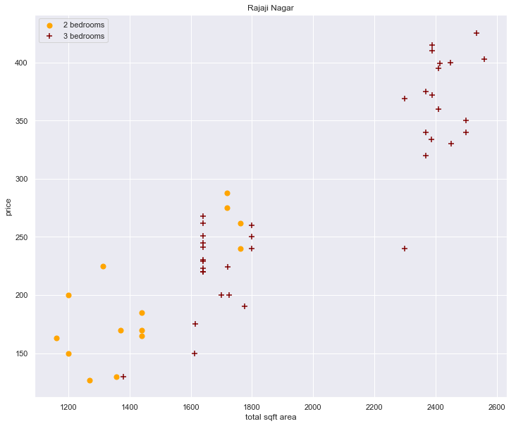
- Around 1700 sqft it seems unusual that 2 bedrooms will be more expensive than a 3 bedroom. This can be another case of outliers that need to be removed.
- let’s look at other observations and see if this trend is common
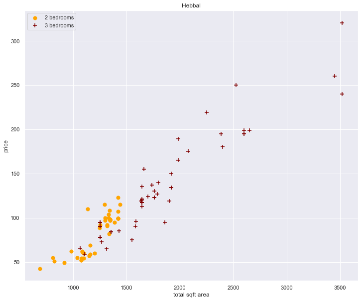
plot_scatter_chart(df4, "Hebbal")
plot_scatter_chart(df4, "Uttarahalli")
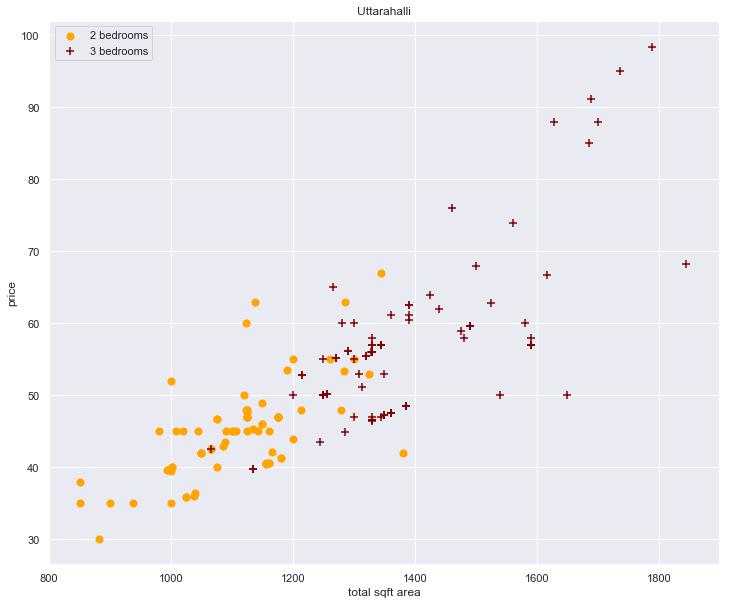
- we can see that these type outlier present themselves more or less commonly.
- we can write a function to remove these outliers
- in other words if the price of a 3 bedroom is less than a 2 bedroom, we can remove those intsances
# this fn performs the above objectives
def remove_bhk_outlier(df):
    exclude_indices = np.array([])
    for location, location_df in df.groupby("location"):
        bhk_stats = {} # generate some stats
        for bhk, bhk_df in location_df.groupby("bhk"):
            bhk_stats[bhk] = {
                "mean": np.mean(bhk_df.price_per_sqft),
                "std": np.std(bhk_df.price_per_sqft),
                "count": bhk_df.shape[0]
            }
        for bhk, bhk_df in location_df.groupby("bhk"):
            stats = bhk_stats.get(bhk-1)
            if stats and stats["count"]>5:
                exclude_indices = np.append(exclude_indices, bhk_df[bhk_df.price_per_sqft < (stats["mean"])].index.values)
    return df.drop(exclude_indices, axis="index")

df5 = remove_bhk_outlier(df4)
df5.shape
(7329, 7)
- now lets see what the function we wrote did!
plot_scatter_chart(df5, "Uttarahalli") # for the prev plot
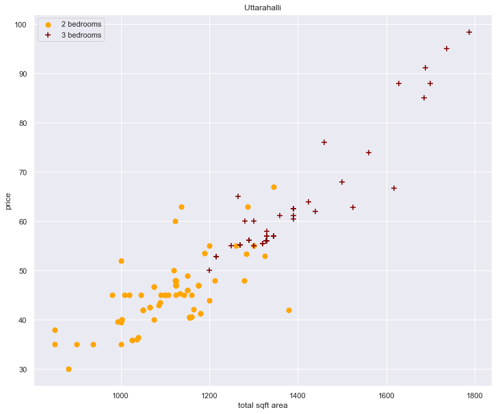
- now there is a descent removal of the outliers
# lets also visualize the number of bathrooms
plt.figure(figsize=(6,5))
plt.hist(df5.bath, rwidth=0.8)
plt.title("bath room counts")
plt.xlabel("number of baths")
plt.ylabel("counts");
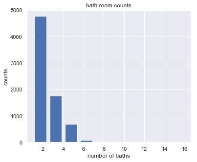
- we can see that most residential properties have 2 - 5 bath rooms with few outliers
- let’s try to remove the bathroom outlier
- for this we shall use the criteria that if the number of bathrooms is more than the number of bedrooms plus 2, we take that as an outlier
df5[df5.bath>df5.bhk+2] # some of the bathroom outliers
| location | size | bhk | total_sqft | bath | price_per_sqft | price | |
|---|---|---|---|---|---|---|---|
| 1626 | Chikkabanavar | 4 Bedroom | 4 | 2460.0 | 7.0 | 3252.032520 | 80.0 |
| 5238 | Nagasandra | 4 Bedroom | 4 | 7000.0 | 8.0 | 6428.571429 | 450.0 |
| 6711 | Thanisandra | 3 BHK | 3 | 1806.0 | 6.0 | 6423.034330 | 116.0 |
| 8411 | other | 6 BHK | 6 | 11338.0 | 9.0 | 8819.897689 | 1000.0 |
- we can see that sometimes we have an apartment with 7 or 8 bathrooms which is unusual
df6 = df5[df5.bath<df5.bhk+2] # removed outliers df
- lets also drop some unneccessary colums like price_per_sqft, and size
df7 = df6[['location', 'bhk', 'total_sqft', 'bath', 'price']]
df7.head()
| location | bhk | total_sqft | bath | price | |
|---|---|---|---|---|---|
| 0 | 1st Block Jayanagar | 4 | 2850.0 | 4.0 | 428.0 |
| 1 | 1st Block Jayanagar | 3 | 1630.0 | 3.0 | 194.0 |
| 2 | 1st Block Jayanagar | 3 | 1875.0 | 2.0 | 235.0 |
| 3 | 1st Block Jayanagar | 3 | 1200.0 | 2.0 | 130.0 |
| 4 | 1st Block Jayanagar | 2 | 1235.0 | 2.0 | 148.0 |
Inferential statistics
Normal distribution
- Here a normal ditribution is a bell-shaped probablity density function (pdf) that is symetric about the mean, showing that data data about the mean are more frequent in occurance than data away from the mean.
- we check the skewness of the target variable by fitting this ditribution and seeing which side it lies (left or right)
plt.rcParams['figure.figsize'] = (11, 9)
plt.xticks(rotation=30)
sns.distplot(df7['price'])
plt.title('Distribution of Target Column')
plt.show()
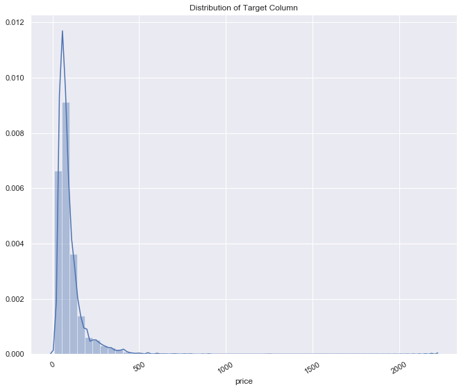
- we can see that the price or target variable is skewed to the right
- the price is not normaly distributed because of outliers
Sample Mean and population Mean
# lets randomly sample the price of 500 houses and compre this to the population mean
samples = np.random.choice(a=df7["price"],size=500)
population_mean = np.mean(df7["price"])

print(f"population mean is: {round(population_mean,3)} \nsample mean is: {round(np.mean(samples),3)}")
population mean is: 96.506
sample mean is: 101.852
- The sample mean is usually not exactly the same as the population mean. This difference can be caused by many factors including poor survey design, biased sampling methods and the randomness inherent to drawing a sample from a population.
Confidence interval
sample_size = 1000
samples = np.random.choice(a=df7["price"],size=sample_size) # let's get a huge sample size

sample_mean = np.mean(samples)

# get critcal z-value
z_critical = stats.norm.ppf(q=0.95) # 95 percentile

pop_std = np.std(df7["price"]) # pop standard dev

# checking the margin of error
margin_of_error = z_critical * (pop_std/math.sqrt(sample_size))

# defining our confidence interval
confidence_interval = (sample_mean - margin_of_error, sample_mean + margin_of_error) # 95% confidence interval

print(f"the critical z value is {z_critical} \nthe 95% CI is {confidence_interval} \nthe true population mean is {population_mean}")
the critical z value is 1.6448536269514722
the 95% CI is (88.57412780284928, 97.69427219715071)
the true population mean is 96.50611846641833
- the true mean is contained within the CI
- confidence interval of 95% would mean that if we take many samples and create confidence intervals for each of them, 95% of our samples’ confidence intervals will contain the true population mean.
- we can also visualize several CI and how they captupre the mean
sample_size = 500

intervals = []
sample_means = []

for sample in range(25):
    sample = np.random.choice(a= df7['price'], size = sample_size)
    sample_mean = sample.mean()
    sample_means.append(sample_mean)

     # Get the z-critical value*
    z_critical = stats.norm.ppf(q = 0.975)

    # Get the population standard deviation
    pop_std = df7['price'].std()

    stats.norm.ppf(q = 0.025)

    margin_of_error = z_critical * (pop_std/math.sqrt(sample_size))

    confidence_interval = (sample_mean - margin_of_error,
                           sample_mean + margin_of_error)

    intervals.append(confidence_interval)


plt.figure(figsize=(13, 9))
plt.errorbar(x=np.arange(0.1, 25, 1),
             y=sample_means,
             yerr=[(top-bot)/2 for top,bot in intervals],
             fmt='o')

plt.hlines(xmin=0, xmax=25,
           y=df7['price'].mean(),
           linewidth=2.0,
           color="red")
plt.title('Confidence Intervals for 25 Trials', fontsize = 20)
plt.show()
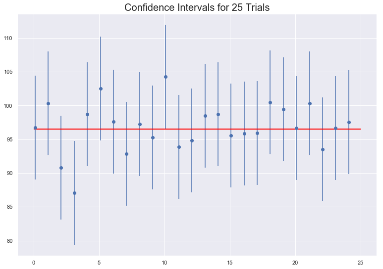
- It is easily visible that 95% of the times the blue lines(the sample mean) overlaps with the red line(the true mean), also 5% of the times it is expected to not overlap with the red line(the true mean).
Hypothesis testing
$\alpha$ = 0.05
$H_0$ : $\mu_0$ = $\mu_1$ equal means in price for all rooms
$H_1$ : $\mu_0$ $\neq$ $\mu_1$
z_statistic, p_value = ztest(x1 = df7[df7["bhk"] == 1 ]['price'], value = df7['price'].mean())
print(f"The p-value is {p_value} and the Z-statistic is {z_statistic}")
The p-value is 0.0 and the Z-statistic is -50.83678679662534
z_statistic, p_value = ztest(x1 = df7[df7["bhk"] == 2 ]['price'], value = df7['price'].mean())
print(f"The p-value is {p_value} and the Z-statistic is {z_statistic}")
The p-value is 0.0 and the Z-statistic is -78.68901645622611
z_statistic, p_value = ztest(x1 = df7[df7["bhk"] == 3 ]['price'], value = df7['price'].mean())
print(f"The p-value is {p_value} and the Z-statistic is {z_statistic}")
The p-value is 1.5976796313461434e-67 and the Z-statistic is 17.362101110701
z_statistic, p_value = ztest(x1 = df7[df7["bhk"] == 4 ]['price'], value = df7['price'].mean())
print(f"The p-value is {p_value} and the Z-statistic is {z_statistic}")
The p-value is 2.7801540796510378e-92 and the Z-statistic is 20.37512315015866
z_statistic, p_value = ztest(x1 = df7[df7["bhk"] == 5 ]['price'], value = df7['price'].mean())
print(f"The p-value is {p_value} and the Z-statistic is {z_statistic}")
The p-value is 1.6776932582667467e-17 and the Z-statistic is 8.514182704074315
z_statistic, p_value = ztest(x1 = df7[df7["bhk"] == 6 ]['price'], value = df7['price'].mean())
print(f"The p-value is {p_value} and the Z-statistic is {z_statistic}")
The p-value is 7.790588657266502e-13 and the Z-statistic is 7.16478999563192
z_statistic, p_value = ztest(x1 = df7[df7["bhk"] == 7 ]['price'], value = df7['price'].mean())
print(f"The p-value is {p_value} and the Z-statistic is {z_statistic}")
The p-value is 0.17705889634431016 and the Z-statistic is 1.3498662280065419
z_statistic, p_value = ztest(x1 = df7[df7["bhk"] == 8 ]['price'], value = df7['price'].mean())
print(f"The p-value is {p_value} and the Z-statistic is {z_statistic}")
The p-value is 0.000813814545059989 and the Z-statistic is 3.348052972037006
z_statistic, p_value = ztest(x1 = df7[df7["bhk"] == 9 ]['price'], value = df7['price'].mean())
print(f"The p-value is {p_value} and the Z-statistic is {z_statistic}")
The p-value is 0.005881467511852069 and the Z-statistic is 2.754317533639393
z_statistic, p_value = ztest(x1 = df7[df7["bhk"] == 10 ]['price'], value = df7['price'].mean())
print(f"The p-value is {p_value} and the Z-statistic is {z_statistic}")
The p-value is nan and the Z-statistic is nan
z_statistic, p_value = ztest(x1 = df7[df7["bhk"] == 11]['price'], value = df7['price'].mean())
print(f"The p-value is {p_value} and the Z-statistic is {z_statistic}")
The p-value is 0.13117985558847922 and the Z-statistic is 1.5094655384150635
z_statistic, p_value = ztest(x1 = df7[df7["bhk"] == 13 ]['price'], value = df7['price'].mean())
print(f"The p-value is {p_value} and the Z-statistic is {z_statistic}")
The p-value is nan and the Z-statistic is nan
z_statistic, p_value = ztest(x1 = df7[df7["bhk"] == 16 ]['price'], value = df7['price'].mean())
print(f"The p-value is {p_value} and the Z-statistic is {z_statistic}")
The p-value is nan and the Z-statistic is nan
- p-value less than $\alpha \le$ 0.05 means that we have enough evidence to reject Null hypothesis of equal means of price in favour of the alternative hypothesis
- interstingly we find that the mean price for most apartments is not the same
- However, the case of 9 and 11 bedroom apartment had p-values greater than 0.05 for which we do not reject the Null hypothesis
- the conclusion is that, the number of rooms has an effect on the price
Predictive Modeling
df7.head()
| location | bhk | total_sqft | bath | price | |
|---|---|---|---|---|---|
| 0 | 1st Block Jayanagar | 4 | 2850.0 | 4.0 | 428.0 |
| 1 | 1st Block Jayanagar | 3 | 1630.0 | 3.0 | 194.0 |
| 2 | 1st Block Jayanagar | 3 | 1875.0 | 2.0 | 235.0 |
| 3 | 1st Block Jayanagar | 3 | 1200.0 | 2.0 | 130.0 |
| 4 | 1st Block Jayanagar | 2 | 1235.0 | 2.0 | 148.0 |
- machine learnint algorithms don’t work with text data. we need to convert the location varaible in a vector using One Hot Encoding
dumies = pd.get_dummies(df7.location, drop_first=True) # sparse matrix
df8 = pd.concat(objs=[df7, dumies], axis="columns")
df8.drop(columns=["location"], inplace=True) # drop column
df8.head()
| bhk | total_sqft | bath | price | 1st Phase JP Nagar | 2nd Phase Judicial Layout | 2nd Stage Nagarbhavi | 5th Block Hbr Layout | 5th Phase JP Nagar | 6th Phase JP Nagar | ... | Vishveshwarya Layout | Vishwapriya Layout | Vittasandra | Whitefield | Yelachenahalli | Yelahanka | Yelahanka New Town | Yelenahalli | Yeshwanthpur | other | |
|---|---|---|---|---|---|---|---|---|---|---|---|---|---|---|---|---|---|---|---|---|---|
| 0 | 4 | 2850.0 | 4.0 | 428.0 | 0 | 0 | 0 | 0 | 0 | 0 | ... | 0 | 0 | 0 | 0 | 0 | 0 | 0 | 0 | 0 | 0 |
| 1 | 3 | 1630.0 | 3.0 | 194.0 | 0 | 0 | 0 | 0 | 0 | 0 | ... | 0 | 0 | 0 | 0 | 0 | 0 | 0 | 0 | 0 | 0 |
| 2 | 3 | 1875.0 | 2.0 | 235.0 | 0 | 0 | 0 | 0 | 0 | 0 | ... | 0 | 0 | 0 | 0 | 0 | 0 | 0 | 0 | 0 | 0 |
| 3 | 3 | 1200.0 | 2.0 | 130.0 | 0 | 0 | 0 | 0 | 0 | 0 | ... | 0 | 0 | 0 | 0 | 0 | 0 | 0 | 0 | 0 | 0 |
| 4 | 2 | 1235.0 | 2.0 | 148.0 | 0 | 0 | 0 | 0 | 0 | 0 | ... | 0 | 0 | 0 | 0 | 0 | 0 | 0 | 0 | 0 | 0 |
5 rows × 245 columns
X = df8.drop(columns="price", axis=1) # features
y = df8["price"] # target
X_train, X_test, y_train, y_test = train_test_split(X,y, test_size=0.20, random_state=67)
lin_reg = LinearRegression()
lin_reg.fit(X_train, y_train)
print(f"Train accuracy: {lin_reg.score(X_train, y_train)} \nTest accuracy: {lin_reg.score(X_test,y_test)}")
Train accuracy: 0.8558407211598535
Test accuracy: 0.8334186940717209
- let try to implement cross validation to see how the model performs
split  = ShuffleSplit(n=X.shape[0],n_iter=5, test_size=0.2,random_state=2)

cross_val_score(estimator=LinearRegression(), X=X, y=y, cv = split)
array([0.86737231, 0.85817913, 0.86058531, 0.79396905, 0.87042283])
- the model give a stable performance
- can we improve on these results?
# now lets build a function to predict the price
def predict_price(location, sqft, bath, bhk):
    loc_idx = np.where(X.columns==location)[0][0] # returns index
    x = np.zeros(len(X.columns))
    x[0]=sqft
    x[1]=bath
    x[2]=bhk
    if loc_idx >= 0:
        x[loc_idx] = 1
    return lin_reg.predict([x])[0]
#
np.where(X.columns=="1st Phase JP Nagar")[0][0]
3
def predict_price(location,sqft,bath,bhk):
    loc_index = np.where(X.columns==location)[0][0]

    x = np.zeros(len(X.columns))
    x[0] = bhk
    x[1] = sqft
    x[2] = bath
    if loc_index >= 0:
        x[loc_index] = 1

    return lin_reg.predict([x])[0]
predict_price('Indira Nagar',1000, 2, 2) # predicting the price of a home in a given location
188.99663978980522
- export model for deployment
import pickle
import json
with open("bangalore_real_estate_estimator.pickle", mode="wb") as f:
    pickle.dump(lin_reg,f)
columns = {
    "data_columns": [col.lower() for col in X.columns]
}

with open("columns.json", mode="w") as f:
    f.write(json.dumps(columns))
- this model is now ready for production!
References
-
[1] https://en.wikipedia.org/wiki/Bangalore.
-
[2] https://www.machinehack.com/course/predicting- house- prices- in-bengaluru/
-
[3] https://www.kaggle.com/amitabhajoy/bengaluru-house-price-data.Sheikh, Wasim, Dash, Mihir, and Sharma, Kshitiz
-
[4] Trends in Residential Marketin Bangalore, India.doi:10.13140/RG.2.2.33967.89768.